

Commercial property managers face increasing pressure to deliver accurate financial projections. Net operating income depends heavily on tight cost controls. Yet, utility expenses remain one of the most volatile line items on any operating statement.
For decades, the standard approach to utility budget forecasting involved a simple formula. Financial teams would pull the previous 12 months of invoices, add three percent to account for inflation, and submit the final figures. This static method works reasonably well during periods of flat energy markets and stable building operations. It fails completely when market dynamics or facility usage patterns change.
Relying solely on historical spend creates major financial exposure. An invoice reflects total dollar amounts, but it hides the underlying drivers of those costs. Energy bills combine consumption volume, peak demand charges, utility delivery rates, supply contract terms, and weather variations into a single dollar figure. When property managers treat that final number as a baseline, they lose visibility into the factors that drive budget variance.
Price volatility in wholesale electricity and natural gas markets makes simple percentage increases risky. Regional transmission organizations continuously adjust capacity charges and grid reliability fees. Local distribution utilities regularly apply for rate hikes with state regulatory commissions. A budget based on last year’s spend plus three percent cannot absorb a fifteen percent jump in capacity costs or a sudden shift in utility delivery rates.
Operational changes further undermine traditional budgeting methods. A shift in tenant occupancy, modified HVAC operating hours, or the installation of high-density equipment alters energy consumption patterns. If a property lost a major tenant last autumn, last year’s winter heating bills reflect space that was fully conditioned for maximum occupancy. Budgeting next year’s spend against those higher usage levels distorts overall financial planning.
Building a reliable forecast requires moving beyond historical spend. Property managers must isolate the variables that drive costs, quantify seasonal risks, and model rate structures accurately. Establishing a precise utility budget protects cash flow, maintains owner trust, and preserves asset valuation.
Building the data foundation for property managers
Accurate financial modeling begins with proper data organization. Property managers must separate total financial spend from raw energy usage metrics. A monthly invoice showing twenty thousand dollars in total charges provides zero context regarding how much electricity or natural gas the building consumed.
To build a defensible baseline, pull at least twenty-four to thirty-six months of detailed billing data. Gather volumetric consumption figures alongside dollar amounts. Track electricity usage in kilowatt-hours and natural gas usage in therms or hundred cubic feet. Capture monthly peak demand measurements, measured in kilowatts, for every electric account.
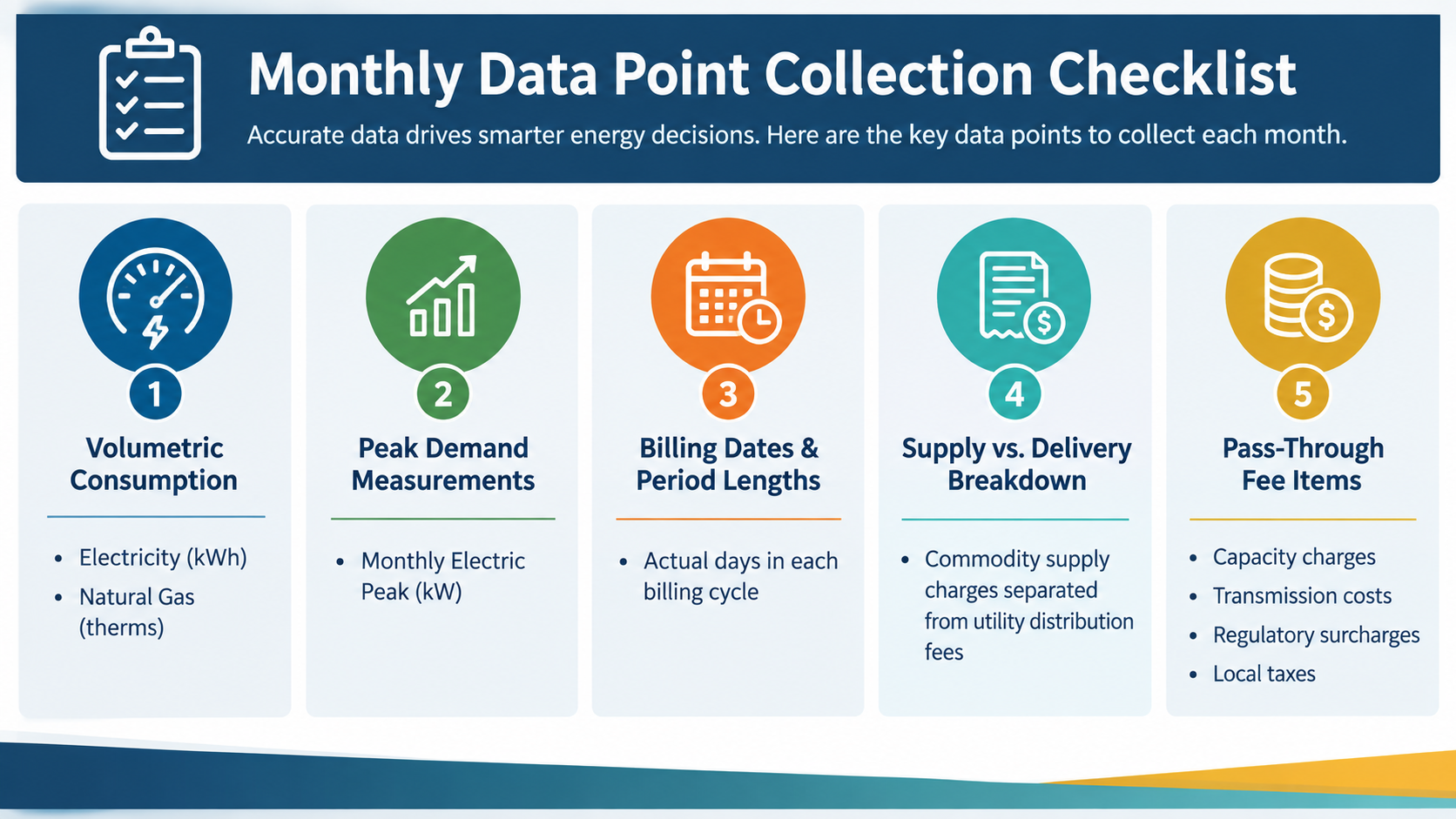
Monthly data point collection checklist
Organizing this data reveals the distinction between base-load usage and weather-sensitive usage. Every commercial building maintains a base load. This represents the energy required to run essential systems regardless of outdoor temperatures, including baseline lighting, security systems, domestic hot water, IT infrastructure, and basic ventilation.
Subtracting estimated base-load consumption from total monthly consumption isolates weather-sensitive peak usage. Summer months reflect cooling loads driven by chillers and rooftop units. Winter months reflect heating loads driven by boilers, furnaces, and resistance heating.
Separating base load from seasonal peak load enables property managers to evaluate efficiency improvements accurately. If a facility installs LED lighting upgrades, the resulting savings will appear in the year-round base load. If the building replaces an aging chiller, the financial return will show up exclusively during peak summer cooling months. Mixing these categories together makes performance tracking impossible.
Account for billing cycle timing differences. Utility billing periods rarely align neatly with calendar months. One invoice might cover twenty-eight days while the next covers thirty-three days. A sudden spike in monthly utility spend might simply reflect five extra days of service rather than higher building usage. Adjusting usage data to standard calendar months establishes a clean baseline for financial modeling.
Incorporating non-price variables into financial models
Once historical consumption data is organized, property managers must adjust the baseline for non-price variables. Weather remains the single largest driver of budget variance in commercial facilities. Comparing raw utility bills from consecutive years without adjusting for weather conditions leads to flawed financial expectations.
Weather normalization removes weather distortion by pairing consumption metrics with local climate data. Heating Degree Days and Cooling Degree Days measure how far outdoor temperatures deviate from a standard baseline, typically sixty-five degrees Fahrenheit. A day with an average temperature of eighty-five degrees generates twenty Cooling Degree Days. A day with an average temperature of forty degrees generates twenty-five Heating Degree Days.
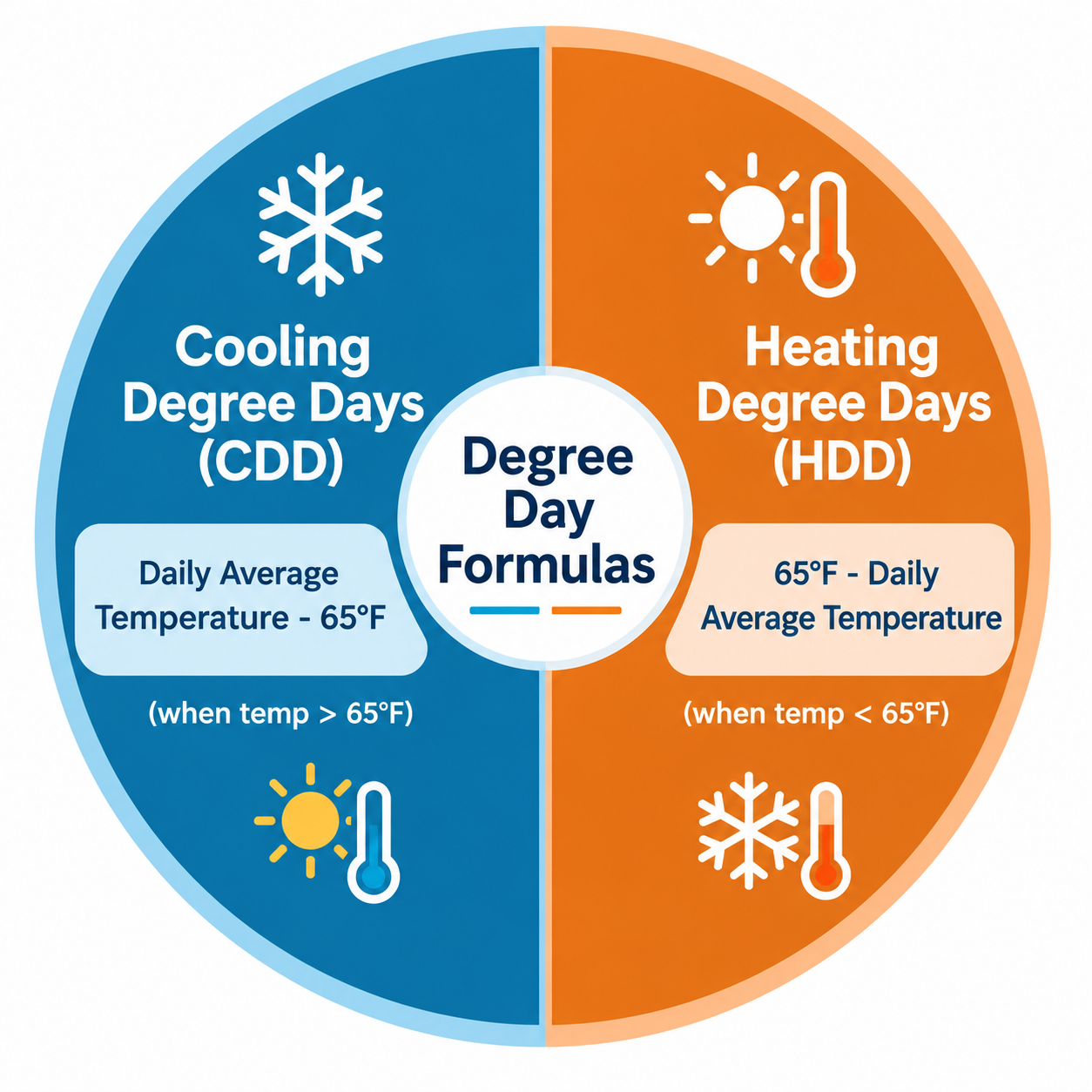
Degree day formulas
Pairing monthly kilowatt-hour consumption with monthly Cooling Degree Days establishes the facility’s weather sensitivity ratio. This calculation shows exactly how many kilowatt-hours the building consumes for every Cooling Degree Day.
If last winter was exceptionally mild, natural gas usage was lower than normal. Budgeting next year’s gas expenses based on that mild season leaves the property exposed if winter temperatures return to historical averages. Normalizing past consumption against ten-year average degree days allows managers to project baseline usage under standard weather conditions.
Operational shifts also require direct adjustments to the baseline model. Building managers must adjust usage calculations whenever operating conditions change.
Changes in tenant lease structures alter utility risk allocation. Converting gross leases to triple-net leases shifts commodity price exposure directly to tenants. Retaining gross lease arrangements means the property owner absorbs every dollar of utility variance. Financial models must mirror these contractual realities so controllers can forecast net cash flow accurately.
Factoring in market structure and rate shifts
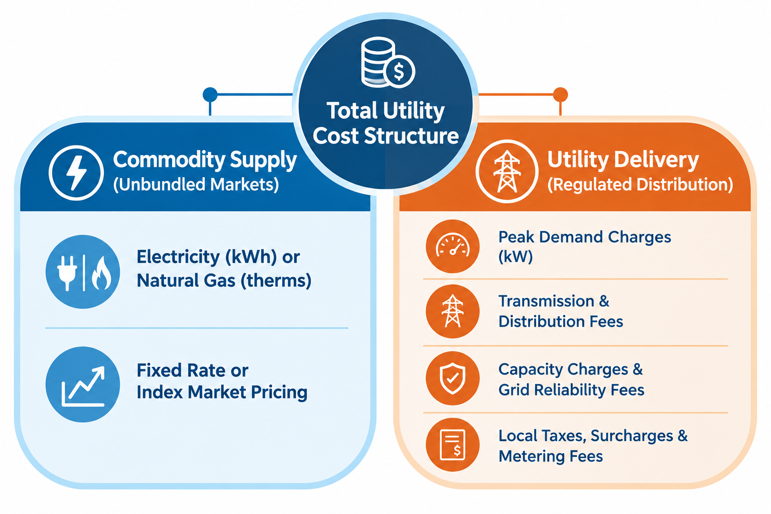
Energy bills consist of two primary cost categories: commodity supply and utility delivery. Commodity supply covers the physical electricity or natural gas consumed. Utility delivery covers the pipelines, wires, transformers, and distribution infrastructure required to move energy to the facility.
In deregulated markets, property managers can contract commodity supply through third-party providers or purchase energy on index markets. A fixed-rate contract offers price stability for the contract duration. An index contract exposes the building directly to wholesale market fluctuations.
Supply contracts contain specific expiration dates. Transition windows represent major budget risks. If a two-year fixed electricity contract expiring in June was locked at six cents per kilowatt-hour, and current wholesale market rates stand at eight cents, the second half of the fiscal year will experience an immediate thirty-three percent increase in commodity costs. Models must account for exact contract end dates rather than applying a single rate across the entire budget year.
Regulated utility distribution rates change independently of supply prices. Local utilities periodically file rate cases with public service commissions to recover infrastructure investment costs. Distribution rate hikes affect every building in the service territory, regardless of third-party supply contracts.
Demand charges represent a massive component of commercial electric bills. Utilities bill demand based on the highest average power draw recorded during a brief interval, usually fifteen minutes, within the billing cycle. A single equipment startup spike can establish a high peak demand charge that elevates electric bills for the entire month. Some utilities enforce ratchet clauses, where setting a high peak demand in summer inflates minimum demand billing for the next eleven months.
Track capacity obligations carefully in deregulated power markets. Electricity markets like PJM, ISO New England, and NYISO calculate a facility’s Capacity Peak Load Contribution based on its power draw during the highest grid-wide demand hours of the preceding summer. This peak load contribution sets the facility’s capacity charge for the following energy year. A building that reduces power draw during grid peak hours lowers its capacity obligations, creating structural savings that must be reflected in the upcoming budget.
Model local taxes, gross receipts taxes, and state environmental surcharges. These pass-through fees increase automatically whenever underlying commodity costs or distribution rates rise.
Master utility budget forecasting to protect NOI
Presenting a single, static dollar figure for annual utility expenses creates false confidence. Weather anomalies, sudden commodity price swings, and unexpected equipment failures make absolute precision impossible. Modern utility budget forecasting relies on presenting dynamic variance ranges backed by clear operational assumptions.
Establishing scenario models prepares ownership and financial executives for potential fluctuations. A standard framework includes three baseline projections:
- Conservative Scenario: Assumes a ten-year average weather profile, steady lease occupancy, and locked commodity contract rates.
- Warm Summer / Cold Winter Scenario: Models a ten percent increase in degree days, testing how severe weather impacts peak cooling and heating expenses.
- Market Exposure Scenario: Models potential supply rate increases at upcoming contract expiration dates alongside projected utility distribution rate filings.
Defining explicit budget assumptions keeps communication clear. When submitting the annual operating plan, outline the exact parameters supporting the numbers. State the assumed degree days, occupancy rates, utility distribution tariff schedules, and contract lock dates.
If actual utility spend diverges from the budget mid-year, executive leadership can immediately identify the cause. If winter temperatures drop twenty percent below historical norms, the controller can attribute the cost overrun directly to weather degree days rather than poor operational management.
Building contingency margins into utility budgets absorbs unexpected market shocks. Rather than adding an arbitrary blanket markup to the final line item, apply targeted risk adjustments to specific volatile components. Hold a tighter margin on fixed supply contracts, but apply a broader contingency range to unhedged natural gas accounts or variable demand charges.
Effective financial modeling transforms utility management from a passive bookkeeping task into a proactive asset strategy. Property managers who master these variables protect property margins and maintain control over facility operating costs.
Take control of utility budget forecasting
Building an accurate, defensible energy budget requires deep analysis of market tariffs, weather adjustments, and building performance metrics. Continuing to rely on outdated budgeting formulas leaves your property portfolio exposed to unmanaged financial risk and budget overruns.
Kb3 Advisors helps commercial property managers, corporate controllers, and asset managers eliminate utility budget surprises. The team analyzes complex tariff structures, audits historical consumption data, evaluates supply contract terms, and builds customized forecasting models that protect net operating income.
Contact Kb3 Advisors today to schedule a comprehensive utility budget and forecast assessment for your commercial portfolio.
Sources
- Commercial Buildings Energy Consumption Survey. eia.gov. Accessed September 10, 2026.
- Benchmark Your Building With Portfolio Manager. energystar.gov. Accessed September 10, 2026.
- Building Performance Database. energy.gov. Accessed September 10, 2026.
